CNN으로 문장 분류하기_180415_18_30.html @ CNN 으로 문장을 분류하는 방법에 대해 살펴보자. 아키텍처와 코드는 각각 Yoon Kim(2014)과 http://emnlp2014.org/papers/pdf/EMNLP2014181.pdf 이곳을 참고했다. http://www.wildml.com/2015/12/implementing-a-cnn-for-text-classification-in-tensorflow/ @ 자연어 처리에 특화된 네트워크 구조? 자연언어는 단어나 표현의 등장 순서가 중요한 sequential data입니다. 아래 예문을 볼까요? {무거운 / *가벼운 / *큰} 침묵 침묵이 {*무겁다}. ‘무거운 침묵’은 고정된 표현형식으로서 ‘정적이 흐르는 상태가 매우 심하다’는 뜻의 collocation 방식으로 쓰인다. 하지만 순서를 바꿔서 ‘침묵이 무겁다’는 표현은 문장 자체가 성립되지 않는 비문이라고 할 수 있다. Only I hit him in the eye yesterday. (No one else did) I only hit him in the eye yesterday. (did not slap him) 영어의 경우 위 예시처럼 단어 등장 순서가 의미 차이를 만드는 경우가 많다. 이렇듯 단어나 표현의 순서는 그 의미 차이를 드러내거나 문장 성립 여부를 결정하는 등 중요한 정보를 함축하고 있다. 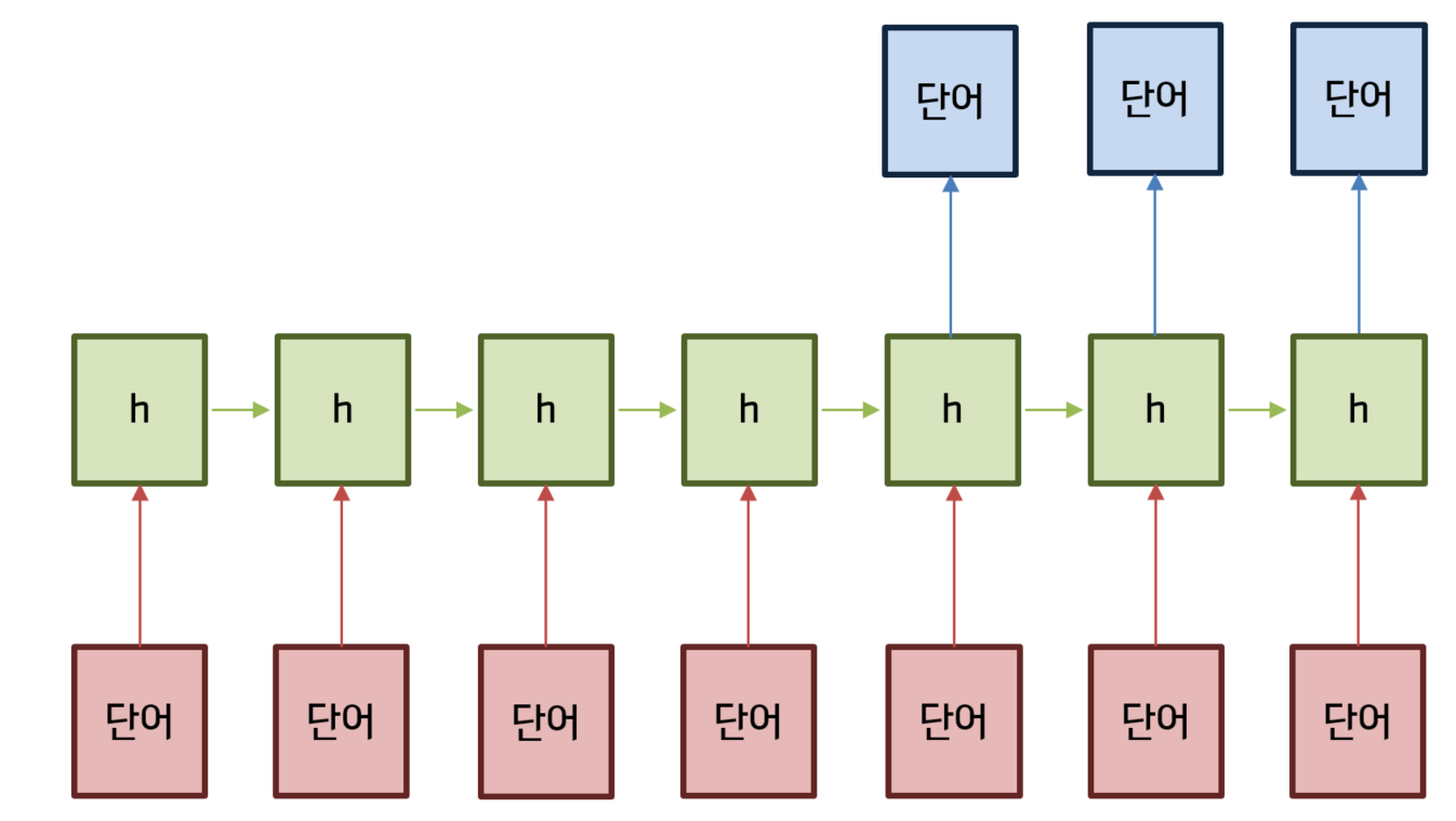@ RNN 이나 CNN은 등장 순서가 중요한 sequential data를 처리하는 데 강점을 지닌 아키텍처이다. RNN의 경우 아래와 같이 입력값을 순차적으로 처리한다. 입력값을 ‘단어’로 바꿔놓고 생각해보면 단어의 등장 순서를 보존하는 형태로 학습이 이뤄지게 됨을 알 수 있다. img cab5a035-db67-42a1-8efd-181568c102f3 @ 그렇다면 CNN은 어떨까? 본래 CNN은 이미지 처리를 하기 위해 만들어진 아키텍처이다. 아래 그림 처럼 filter 가 움직이면서 이미지의 지역적인 정보를 추출, 보존하는 형태로 학습이 이뤄지게 된다. img e0627aa9-fddf-4328-a590-03d4217e8523.gif @ CNN을 텍스트 처리에 응용한 연구가 Yoon Kim(2014) 이다. 이미지 처리를 위한 CNN의 필터(9칸짜리 노란색 박스)가 이미지의 지역적인 정보를 추출하는 역할을 한다면, 텍스트 CNN의 필터는 텍스트의 지역적인 정보, 즉 단어 등장순서/문맥 정보를 보존한다는 것이다. 이를 도식화하면 아래 움짤과 같다. img a0157374-3736-4edc-b70b-cb0e84df9a78.gif 한 문장당 단어 수는 총 n개(아래 코드에서 변수명: sequence_length) 이다. 이 단어들 각각은 p차원(변수명: embedding_size) 의 벡터이다. 붉은색 박스는 필터를 의미한다. 필터의 크기는 2로써 한번에 단어 2개씩을 보게 된다. 이 필터는 문장에 등장한 단어들을 출현 순서대로 슬라이딩 해가면서, 문장의 지역적인 정보를 보존하게 된다. 필터의 크기가 1이라면 Unigram, 2라면 Bigram, 3이면 Trigram, 이런 식으로 필터의 크기를 조절함으로써 다양한 N-gram 모델을 만들어낼 수 있다. @ RNN은 단어 입력값을 순서대로 처리함으로써, CNN은 문장의 지역 정보를 보존함으로써, 단어/표현의 등장순서를 학습에 반영하는 아키텍처라 할 수 있겠다. RNN과 CNN이 자연언어처리 분야에서도 각광받고 있는 이유이기도 하다. 이 글에서 설명하지 않았지만 Recursive Neural Networks도 단어/표현의 등장순서를 학습에 반영하는 구조이다. Recursive Neural Networks의 자세한 내용을 보시려면 이곳을 참고하면된다. https://ratsgo.github.io/deep%20learning/2017/04/03/recursive/ 아울러 CNN의 역전파(backpropagation) 등 학습방식에 관심이 있으시면 이곳을 참고하면된다. https://ratsgo.github.io/deep%20learning/2017/04/05/CNNbackprop/ RNN의 어플리케이션 사례를 보시려면 이곳을 참고하면 된다. https://ratsgo.github.io/natural%20language%20processing/2017/03/12/s2s/ @ CNN을 활용한 문장 분류 아키텍처 Yoon Kim(2014)의 아키텍처는 아래와 같다. img 2516f0b8-e315-4e33-8f61-7ceca45b2faa 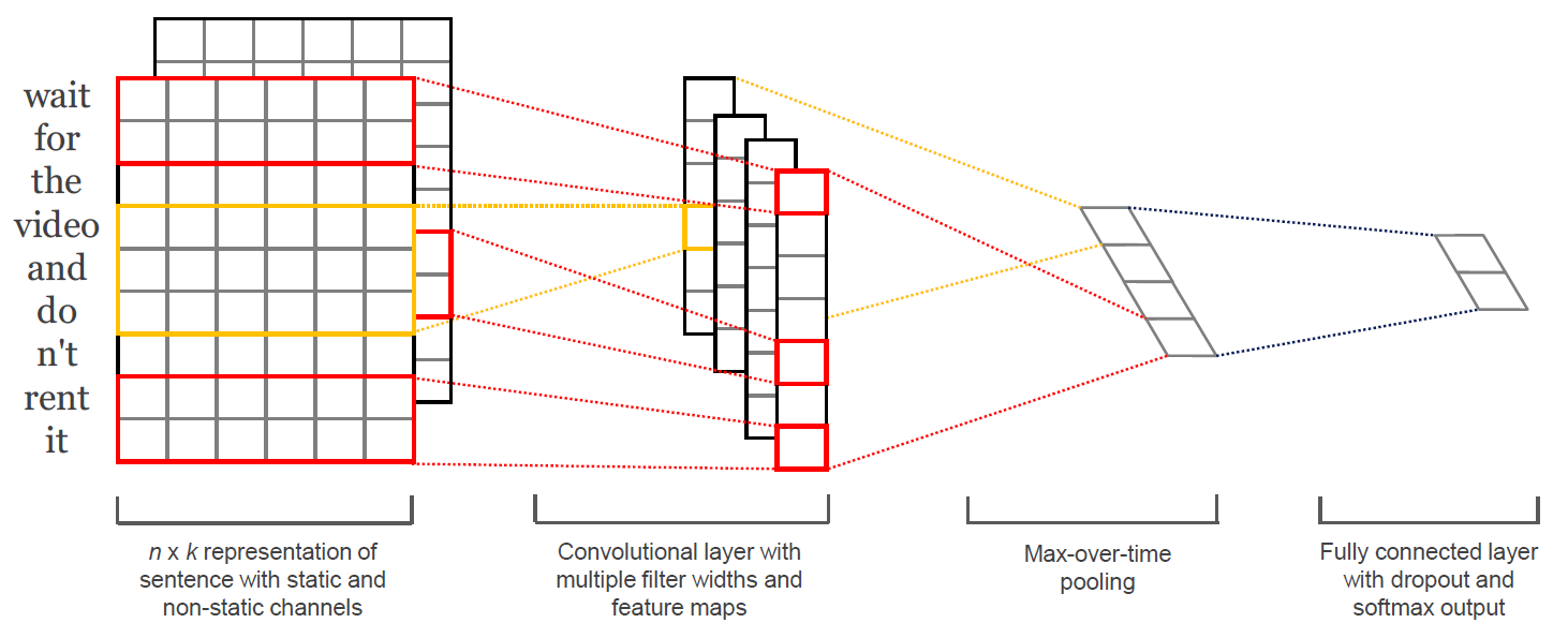이 논문은 영화 리뷰 사이트에 게시된 댓글과 평점 정보를 이용해, 각 리뷰가 긍정인지 부정인지 분류하는 모델을 만들고자 했다. n개의 단어로 이뤄진 하나의 리뷰 문장에서 각 단어를 k차원의 행벡터로 임베딩하여 (k,n) matrix 를 만든다. 단어를 벡터로 임베딩하기 위해서는 Word2Vec이나 GloVe처럼 distributed representation을 쓸 수 있다. 혹은, 한단어 행벡터의 초기값을 랜덤으로 준 뒤, 이를 다른 파라메터들처럼 학습 과정에서 조금씩 업데이트해서 사용하는 방법을 쓸 수도 있다. 한편 위 그림을 보면 CNN 필터의 크기는 2와 3인데, 각각 Bigram, Trigram 모델을 뜻한다고 볼 수 있다. 이후 필터 개수만큼의 feature map을 만들고, Max-pooling 과정을 거쳐 클래스 개수(긍정 혹은 부정:2개)만큼의 스코어를 출력하는 네트워크 구조이다. @ 영화리뷰를 숫자로 바꾸기 텐서플로우 코드로 구현된 이 아키텍처를 한국어 영화 리뷰에 적용해 보기로 했다. 우선 영화 리뷰 품질이 국내에서 가장 좋은 것으로 평가받는 왓챠에서, 댓글과 평점 데이터 657만2288건을 모았다. 스크래핑한 데이터는 아래와 같다. 알프레도는 필름을 통해 인생과 사랑에 대해서 얘기하고자 했던것같다. 그 무수한 날들을 거치면서 항상 전진해야했던 토토에 비해 영화는 항상 향수를 자극시키며 그 자리에 계속 있었다. 많은 오고가는 흐릿한 생각들 끝에 내가 생각하는 영화는 정말 사랑과도 같다. 이해할수도 설명할수도 없는 그 느낌. 이 영화를 통해 영화를 더욱 사랑하게되었다, 5.0 고마워요 알프레도, 4.0 나머지 별 반개는 감독판을 보는 날에, 4.5 영화가 주는 감동이란..., 4.5 뭘 얘기하고 싶은건데?, 2.0 @ 우선 "CNN 문장분류 app" 아키텍처의 입력값과 출력값을 만들어야 한다. 입력 데이터를 만들어 보자. 이 글에서는 Word2Vec 같은 distributed representation을 쓰지 않고, 단어벡터를 랜덤하게 초기화한 뒤 이를 학습과정에서 업데이트하면서 쓰는 방법을 채택했다. 이런 방식을 사용하기 위해서는 위 리뷰 텍스트 문장을 숫자들(각 단어의 ID)의 나열로 변환해야 한다. 그런데 단어들이 너무 많으면 메모리 문제로 학습 자체가 불가능해지므로, 전체 단어 숫자를 줄일 필요가 있다. 이를 위해 문장을 띄어쓰기 기준으로 어절로 나눈다. 어절 처음 두 글자만 자른다. 바꿔 말하면 아래 단어들을 모두 한 단어로 보는 방식이다. 잘어울리는 잘어울렸다 잘어울리네요 잘어울리는데 잘어울림 잘어울려요 잘어울리고 잘어울렸는데 잘어울렸음 잘어울린다 이 방식을 적용하면 말뭉치에 등장하는 전체 단어수(변수명: vocab_size)를, 아무런 처리를 하지 않았던 기존 대비 4분의 1로 줄일 수 있다. 이후 단어별로 ID를 부여해 사전을 만든다. 이 사전을 가지고 각 리뷰를 ID(숫자)들의 나열로 바꾸는 것이다. {‘가’: 0, ‘가가’: 1, ‘가감’: 2, (중략) ‘잘어’: 10004, (하략) } 이제 출력(정답) 데이터를 살펴볼까? 왓챠 평점은 5점 만점인데 2.5점보다 높으면 긍정([1,0])을, 2.5점보다 낮으면 부정([0,1]) 범주를 부여했다. 지금까지 설명한 방식을 적용해 입력값과 출력값을 만든 결과의 예시는 아래와 같다. 고마워요 알프레도 (하략), 4.0 [[502, 3101, ......], [1,0]] 영화가 주는 감동이란 (하략), 4.5 [[2022, 3043, 301, ...], [1,0]] 뭘 얘기하고 싶은건데? (하략), 2.0 [[1005, 2206, 1707, ...], [0,1]] @ Lookup 테이블 구축 지금까지 우리가 만든 입력값은 아래 그림에서 빨간색 테두리 박스에 대응된다. 다시 말해 빨간색 테두리 박스는 한 문장의 길이(변수명:sequence_length)에 해당하는 숫자만큼의 단어 ID들의 나열이다. 이번 글에서는 Word2Vec을 쓰지 않고 단어벡터를 만들기로 했다. 대신 커다란 Lookup 테이블(아래 그림에서 파란색 테두리 박스)을 만들것이다. 이 테이블의 크기는, 전체 단어의 갯수(변수명:vocab_size) * 사용자가 지정한 한단어행벡터의 차원수(변수명:embedding_size) 이다. 파란색 테두리 박스의 한단어행벡터들은 개별 단어 ID에 대응하는 벡터이다. 초기값은 랜덤하게 설정한다. 이후 학습 과정에서 문장 분류를 가장 잘하는 방식으로 조금씩 업데이트된다. 지금까지 리뷰문장을 단어 ID들의 나열로 바꿨다. ID에 해당하는 한단어행벡터도 만들었다. 이제 단어 ID들 각각을 벡터로 바꿔주기만 하면 된다. 방법은 쉽다. 파란색 Lookup 테이블에서 단어 ID에 해당하는 한단어행벡터를 참조해서 가져오기만 하면 된다. 그 결과는 바로 아래 그림의 보라색 테두리 박스이다. 이 박스의 크기는 (한문장길이 sequence_length * 사용자가 지정한 한단어행벡터의 차원수 embedding_size)가 된다. img 7a0681cd-6179-43af-b91a-44a35aac4c8e @ 위에서 논의한 내용을 텐서플로우 코드로 표현하면 다음과 같다. W = tf.Variable(tf.random_uniform([vocab_size, embedding_size], -1.0, 1.0), name="W") # 최종 결과물인 보라색 박스에 대응하는 변수명은 embedded_chars 이다 # 차원수: [sequence length, embedding size] embedded_chars = tf.nn.embedding_lookup(W, input_x) # 여기에 conv2d() 가 요구하는 차원수로 만들어주기 위해 차원을 하나 추가해 준다. # 차원수 : [sequence length * embedding size * 1] embedded_chars_expanded = tf.expand_dims(embedded_chars, -1) @ Conv Layer 만들기 embedded_chars_expanded 는 배치(batch) 단위로 CNN에 들어가게 된다. 배치를 반영한 입력값의 차원수는 [batch_size, sequence_length, embedding_size, channel_size] 가 된다. 그런데 제가 실험한 CNN 구조에선 채널수를 1로 설정하여서 결과적으로, [batch_size, sequence_length, embedding_size, 1] 이 된다. 이제 필터의 차원수를 살펴보겠다. 아래 그림을 보면 알겠지만, 필터의 너비는 embedding_size (dimension of 한단어 행벡터) 입니다. 높이는 filter_size 인데, 만약 2라면 Bigram, 3이라면 Trigram 모델이 될 것이다. 채널수는 1로 고정했다. img c9f295cb-c658-46ef-bb34-5b73bc7a225a # 이를 종합해 텐서플로우가 요구하는 문법으로 필터의 shape 을 정의하면 다음과 같다. filter_shape = [filter_size, embedding_size, 1, num_filters] @ 이제, 텐서플로우 구현의 핵심인 convolution layer 를 만드는 부분을 보자. # 여기서 "입력값" 과 "필터의 가중치" 는 각각 embedded_chars_expanded, W 이다 # 필터가 입력값을 볼 때 strides 는 [1, 1, 1, 1] 로 하고 "엣지 패딩" 없이 문장을 슬라이딩하라는 뜻이다 conv = tf.nn.conv2d(self.embedded_chars_expanded, W, strides=[1, 1, 1, 1], padding="VALID", name="conv") h = tf.nn.relu(tf.nn.bias_add(conv, b), name="relu") [1, 1, 1, 1] 의 의미는? 텐서플로우 문서를 보면 strides값은, [batch_size, input_height, input_width, input_channels] 순서로 지정하라고 정의돼 있다. 보폭이 [1, 1, 1, 1]이라는 건 배치데이터 하나씩, 단어 하나씩 슬라이딩하면서 보라는 의미이다. 그런데 여기서 input_width 와 input_channels 는 큰 의미가 없다. 왜냐하면 우리는 입력값의 너비와 필터의 너비를 embedding_size 로 같게 설정했고, 채널수는 1로 모두 고정했기 때문이다. 바꿔 말하면 보폭 [1, 1, 1, 1] 중 뒤의 두 값은 입력데이터와 필터가 같은 값을 지니기 때문에, 슬라이딩할 수 있는 여유 공간이 없어 무의미하다는 뜻이다. 이렇게 convolution 를 적용한 뒤, 텐서의 차원수는 [batch_size,sequence_length-filter_size+1,1,num_filters] 가 된다. 첫번째 요소로 batch_size 가 나오는 건 직관적으로 이해 가능할 것이다. 나머지 차원수에 대해서는 텐서플로우 공식문서를 확인하시면 빠르게 이해할 수 있다. 이후 ReLU를 써서 비선형성(non-linearity)을 확보한다. @ 이제, Max-pooling 하는 부분을 보겠다. 여기서 핵심은 ksize 이다. Max-pooling 하는 영역의 크기이다. 예컨대 ksize 가 [1, 2, 2, 1] 이라면, 배치데이터/채널별로 가로, 세로 두 칸씩 움직이면서 Max-pooling 하라는 지시이다. Max-pooling 이 적용된 후의 텐서 차원수는 [batch_size, 1, 1, num_filters] 가 된다. pooled=tf.nn.max_pool(\ h\ ,ksize=[1, sequence_length - filter_size + 1, 1, 1]\ ,strides=[1, 1, 1, 1]\ ,padding='VALID'\ ,name="pool") @ 이후엔 Max-pooling 한 결과물을 합친다. Full-connected layer 를 통과시켜 각 클래스에 해당하는 스코어를 낸다. cross entropy 를 써서 loss 를 구한다. Backpropagation 을 수행해 필터의 가중치 등 파라메터들을 업데이트하는 일반적인 과정을 거친다. 여기서 특이한 점은 단어벡터의 모음인 Lookup 테이블도 학습과정에서 같이 업데이트한다는 사실이다. @ 코드 공유 지금까지 이야기한 내용을 바탕으로 이곳을 참고해 커스터마이징한 코드는 아래와 같다. http://www.wildml.com/2015/12/implementing-a-cnn-for-text-classification-in-tensorflow/ import os import time import datetime from tensorflow import flags import tensorflow as tf import numpy as np import cnn_tool as tool class TextCNN(object): """ A CNN for text classification. Uses an embedding layer, followed by a convolutional, max-pooling and softmax layer. <Parameters> - sequence_length: 최대 문장 길이 - num_classes: 클래스 개수 - vocab_size: 등장 단어 수 - embedding_size: 각 단어에 해당되는 임베디드 벡터의 차원 - filter_sizes: convolutional filter들의 사이즈 (= 각 filter가 몇 개의 단어를 볼 것인가?) (예: "3, 4, 5") - num_filters: 각 filter size 별 filter 수 - l2_reg_lambda: 각 weights, biases에 대한 l2 regularization 정도 """ def __init__( self, sequence_length, num_classes, vocab_size, embedding_size, filter_sizes, num_filters, l2_reg_lambda=0.0): # Placeholders for input, output and dropout self.input_x = tf.placeholder(tf.int32, [None, sequence_length], name="input_x") self.input_y = tf.placeholder(tf.float32, [None, num_classes], name="input_y") self.dropout_keep_prob = tf.placeholder(tf.float32, name="dropout_keep_prob") # Keeping track of l2 regularization loss (optional) l2_loss = tf.constant(0.0) # Embedding layer """ <Variable> - W: 각 단어의 임베디드 벡터의 성분을 랜덤하게 할당 """ with tf.device('/gpu:0'), tf.name_scope("embedding"): #with tf.device('/cpu:0'), tf.name_scope("embedding"): W = tf.Variable( tf.random_uniform([vocab_size, embedding_size], -1.0, 1.0), name="W") self.embedded_chars = tf.nn.embedding_lookup(W, self.input_x) self.embedded_chars_expanded = tf.expand_dims(self.embedded_chars, -1) # Create a convolution + maxpool layer for each filter size pooled_outputs = [] for i, filter_size in enumerate(filter_sizes): with tf.name_scope("conv-maxpool-%s" % filter_size): # Convolution Layer filter_shape = [filter_size, embedding_size, 1, num_filters] W = tf.Variable(tf.truncated_normal(filter_shape, stddev=0.1), name="W") b = tf.Variable(tf.constant(0.1, shape=[num_filters]), name="b") conv = tf.nn.conv2d( self.embedded_chars_expanded, W, strides=[1, 1, 1, 1], padding="VALID", name="conv") # Apply nonlinearity h = tf.nn.relu(tf.nn.bias_add(conv, b), name="relu") # Maxpooling over the outputs pooled = tf.nn.max_pool( h, ksize=[1, sequence_length - filter_size + 1, 1, 1], strides=[1, 1, 1, 1], padding='VALID', name="pool") pooled_outputs.append(pooled) # Combine all the pooled features num_filters_total = num_filters * len(filter_sizes) self.h_pool = tf.concat(3, pooled_outputs) self.h_pool_flat = tf.reshape(self.h_pool, [-1, num_filters_total]) # Add dropout with tf.name_scope("dropout"): self.h_drop = tf.nn.dropout(self.h_pool_flat, self.dropout_keep_prob) # Final (unnormalized) scores and predictions with tf.name_scope("output"): W = tf.get_variable( "W", shape=[num_filters_total, num_classes], initializer=tf.contrib.layers.xavier_initializer()) b = tf.Variable(tf.constant(0.1, shape=[num_classes]), name="b") l2_loss += tf.nn.l2_loss(W) l2_loss += tf.nn.l2_loss(b) self.scores = tf.nn.xw_plus_b(self.h_drop, W, b, name="scores") self.predictions = tf.argmax(self.scores, 1, name="predictions") # Calculate Mean cross-entropy loss with tf.name_scope("loss"): losses = tf.nn.softmax_cross_entropy_with_logits(self.scores, self.input_y) self.loss = tf.reduce_mean(losses) + l2_reg_lambda * l2_loss # Accuracy with tf.name_scope("accuracy"): correct_predictions = tf.equal(self.predictions, tf.argmax(self.input_y, 1)) self.accuracy = tf.reduce_mean(tf.cast(correct_predictions, "float"), name="accuracy") # data loading data_path = 'C:/Users/ratsgo/GoogleDrive/내폴더/textmining/data/watcha_movie_review_spacecorrected.csv' contents, points = tool.loading_rdata(data_path, eng=True, num=True, punc=False) contents = tool.cut(contents,cut=2) # tranform document to vector max_document_length = 200 x, vocabulary, vocab_size = tool.make_input(contents,max_document_length) print('사전단어수 : %s' % (vocab_size)) y = tool.make_output(points,threshold=2.5) # divide dataset into train/test set x_train, x_test, y_train, y_test = tool.divide(x,y,train_prop=0.8) # Model Hyperparameters flags.DEFINE_integer("embedding_dim", 128, "Dimensionality of embedded vector (default: 128)") flags.DEFINE_string("filter_sizes", "3,4,5", "Comma-separated filter sizes (default: '3,4,5')") flags.DEFINE_integer("num_filters", 128, "Number of filters per filter size (default: 128)") flags.DEFINE_float("dropout_keep_prob", 0.5, "Dropout keep probability (default: 0.5)") flags.DEFINE_float("l2_reg_lambda", 0.1, "L2 regularization lambda (default: 0.0)") # Training parameters flags.DEFINE_integer("batch_size", 64, "Batch Size (default: 64)") flags.DEFINE_integer("num_epochs", 10, "Number of training epochs (default: 200)") flags.DEFINE_integer("evaluate_every", 100, "Evaluate model on dev set after this many steps (default: 100)") flags.DEFINE_integer("checkpoint_every", 100, "Save model after this many steps (default: 100)") flags.DEFINE_integer("num_checkpoints", 5, "Number of checkpoints to store (default: 5)") # Misc Parameters flags.DEFINE_boolean("allow_soft_placement", True, "Allow device soft device placement") flags.DEFINE_boolean("log_device_placement", False, "Log placement of ops on devices") FLAGS = tf.flags.FLAGS FLAGS._parse_flags() print("\nParameters:") for attr, value in sorted(FLAGS.__flags.items()): print("{}={}".format(attr.upper(), value)) print("") # 3. train the model and test with tf.Graph().as_default(): sess = tf.Session() with sess.as_default(): cnn = TextCNN(sequence_length=x_train.shape[1], num_classes=y_train.shape[1], vocab_size=vocab_size, embedding_size=FLAGS.embedding_dim, filter_sizes=list(map(int, FLAGS.filter_sizes.split(","))), num_filters=FLAGS.num_filters, l2_reg_lambda=FLAGS.l2_reg_lambda) # Define Training procedure global_step = tf.Variable(0, name="global_step", trainable=False) optimizer = tf.train.AdamOptimizer(1e-3) grads_and_vars = optimizer.compute_gradients(cnn.loss) train_op = optimizer.apply_gradients(grads_and_vars, global_step=global_step) # Keep track of gradient values and sparsity (optional) grad_summaries = [] for g, v in grads_and_vars: if g is not None: grad_hist_summary = tf.summary.histogram("{}".format(v.name), g) sparsity_summary = tf.summary.scalar("{}".format(v.name), tf.nn.zero_fraction(g)) grad_summaries.append(grad_hist_summary) grad_summaries.append(sparsity_summary) grad_summaries_merged = tf.summary.merge(grad_summaries) # Output directory for models and summaries timestamp = str(int(time.time())) out_dir = os.path.abspath(os.path.join(os.path.curdir, "runs", timestamp)) print("Writing to {}\n".format(out_dir)) # Summaries for loss and accuracy loss_summary = tf.summary.scalar("loss", cnn.loss) acc_summary = tf.summary.scalar("accuracy", cnn.accuracy) # Train Summaries train_summary_op = tf.summary.merge([loss_summary, acc_summary, grad_summaries_merged]) train_summary_dir = os.path.join(out_dir, "summaries", "train") train_summary_writer = tf.summary.FileWriter(train_summary_dir, sess.graph) # Dev summaries dev_summary_op = tf.summary.merge([loss_summary, acc_summary]) dev_summary_dir = os.path.join(out_dir, "summaries", "dev") dev_summary_writer = tf.summary.FileWriter(dev_summary_dir, sess.graph) # Checkpoint directory. Tensorflow assumes this directory already exists so we need to create it checkpoint_dir = os.path.abspath(os.path.join(out_dir, "checkpoints")) checkpoint_prefix = os.path.join(checkpoint_dir, "model") if not os.path.exists(checkpoint_dir): os.makedirs(checkpoint_dir) saver = tf.train.Saver(tf.global_variables(), max_to_keep=FLAGS.num_checkpoints) # Initialize all variables sess.run(tf.global_variables_initializer()) def train_step(x_batch, y_batch): """ A single training step """ feed_dict = { cnn.input_x: x_batch, cnn.input_y: y_batch, cnn.dropout_keep_prob: FLAGS.dropout_keep_prob } _, step, summaries, loss, accuracy = sess.run( [train_op, global_step, train_summary_op, cnn.loss, cnn.accuracy], feed_dict) time_str = datetime.datetime.now().isoformat() print("{}: step {}, loss {:g}, acc {:g}".format(time_str, step, loss, accuracy)) train_summary_writer.add_summary(summaries, step) def dev_step(x_batch, y_batch, writer=None): """ Evaluates model on a dev set """ feed_dict = { cnn.input_x: x_batch, cnn.input_y: y_batch, cnn.dropout_keep_prob: 1.0 } step, summaries, loss, accuracy = sess.run( [global_step, dev_summary_op, cnn.loss, cnn.accuracy], feed_dict) time_str = datetime.datetime.now().isoformat() print("{}: step {}, loss {:g}, acc {:g}".format(time_str, step, loss, accuracy)) if writer: writer.add_summary(summaries, step) def batch_iter(data, batch_size, num_epochs, shuffle=True): """ Generates a batch iterator for a dataset. """ data = np.array(data) data_size = len(data) num_batches_per_epoch = int((len(data) - 1) / batch_size) + 1 for epoch in range(num_epochs): # Shuffle the data at each epoch if shuffle: shuffle_indices = np.random.permutation(np.arange(data_size)) shuffled_data = data[shuffle_indices] else: shuffled_data = data for batch_num in range(num_batches_per_epoch): start_index = batch_num * batch_size end_index = min((batch_num + 1) * batch_size, data_size) yield shuffled_data[start_index:end_index] # Generate batches batches = batch_iter( list(zip(x_train, y_train)), FLAGS.batch_size, FLAGS.num_epochs) testpoint = 0 # Training loop. For each batch... for batch in batches: x_batch, y_batch = zip(*batch) train_step(x_batch, y_batch) current_step = tf.train.global_step(sess, global_step) if current_step % FLAGS.evaluate_every == 0: if testpoint + 100 < len(x_test): testpoint += 100 else: testpoint = 0 print("\nEvaluation:") dev_step(x_test[testpoint:testpoint+100], y_test[testpoint:testpoint+100], writer=dev_summary_writer) print("") if current_step % FLAGS.checkpoint_every == 0: path = saver.save(sess, checkpoint_prefix, global_step=current_step) print("Saved model checkpoint to {}\n".format(path)) view rawcnn_sentence_classification.py hosted with ❤ by GitHub https://gist.github.com/ratsgo/7ff405f582437dbf96216dd940917427#file-cnn_sentence_classification-py @ 위 코드에 쓰인 입력데이터 전처리용 코드는 다음과 같습니다. import numpy as np import pandas as pd import re import tensorflow as tf import random #################################################### # cut words function # #################################################### def cut(contents, cut=2): results = [] for content in contents: words = content.split() result = [] for word in words: result.append(word[:cut]) results.append(' '.join([token for token in result])) return results #################################################### # divide train/test set function # #################################################### def divide(x, y, train_prop): random.seed(1234) x = np.array(x) y = np.array(y) tmp = np.random.permutation(np.arange(len(x))) x_tr = x[tmp][:round(train_prop * len(x))] y_tr = y[tmp][:round(train_prop * len(x))] x_te = x[tmp][-(len(x)-round(train_prop * len(x))):] y_te = y[tmp][-(len(x)-round(train_prop * len(x))):] return x_tr, x_te, y_tr, y_te #################################################### # making input function # #################################################### def make_input(documents, max_document_length): # tensorflow.contrib.learn.preprocessing 내에 VocabularyProcessor라는 클래스를 이용 # 모든 문서에 등장하는 단어들에 인덱스를 할당 # 길이가 다른 문서를 max_document_length로 맞춰주는 역할 vocab_processor = tf.contrib.learn.preprocessing.VocabularyProcessor(max_document_length) # 객체 선언 x = np.array(list(vocab_processor.fit_transform(documents))) ### 텐서플로우 vocabulary processor # Extract word:id mapping from the object. # word to ix 와 유사 vocab_dict = vocab_processor.vocabulary_._mapping # Sort the vocabulary dictionary on the basis of values(id). sorted_vocab = sorted(vocab_dict.items(), key=lambda x: x[1]) # Treat the id's as index into list and create a list of words in the ascending order of id's # word with id i goes at index i of the list. vocabulary = list(list(zip(*sorted_vocab))[0]) return x, vocabulary, len(vocab_processor.vocabulary_) #################################################### # make output function # #################################################### def make_output(points, threshold): results = np.zeros((len(points),2)) for idx, point in enumerate(points): if point > threshold: results[idx,0] = 1 else: results[idx,1] = 1 return results #################################################### # check maxlength function # #################################################### def check_maxlength(contents): max_document_length = 0 for document in contents: document_length = len(document.split()) if document_length > max_document_length: max_document_length = document_length return max_document_length #################################################### # loading function # #################################################### def loading_rdata(data_path, eng=True, num=True, punc=False): # R에서 title과 contents만 csv로 저장한걸 불러와서 제목과 컨텐츠로 분리 # write.csv(corpus, data_path, fileEncoding='utf-8', row.names=F) corpus = pd.read_table(data_path, sep=",", encoding="utf-8") corpus = np.array(corpus) contents = [] points = [] for idx,doc in enumerate(corpus): if isNumber(doc[0]) is False: content = normalize(doc[0], english=eng, number=num, punctuation=punc) contents.append(content) points.append(doc[1]) if idx % 100000 is 0: print('%d docs / %d save' % (idx, len(contents))) return contents, points def isNumber(s): try: float(s) return True except ValueError: return False view rawcnn_tool.py hosted with ❤ by GitHub https://gist.github.com/ratsgo/d5c43d40be348987c69466c81edb3904#file-cnn_tool-py @ 제가 실험한 결과도 간략히 소개합니다. 제가 선택한 하이퍼파라메터 조합은 아래와 같습니다. embedding_size = 128 filter_sizes = 3,4,5 num_filters = 128 dropout_keep_prob = 0.5 batch_size = 64 max_document_length = 100 우선 왓챠에서 모은 댓글과 평점 데이터 657만2288건 가운데 80%를 학습데이터, 20%를 검증데이터로 분리했습니다. 학습에 쓰지 않은 검증데이터에 대한 예측 결과(단순정확도)는 step수가 3만회를 넘어가면서 85% 내외로 수렴하는 모습을 보였습니다. 그 결과는 다음과 같습니다. step 37600, loss 0.401777, acc 0.87 step 41500, loss 0.347608, acc 0.85 step 47000, loss 0.384077, acc 0.84 step 51000, loss 0.30739, acc 0.86 step 53800, loss 0.328676, acc 0.82 @ 마치며 이상으로 CNN을 활용한 문장 분류 모델을 살펴보았습니다. CNN은 지역 정보를 보존한다는 점에서 순차적인 데이터 처리에 강점을 지닌 RNN과 더불어 자연언어처리 분야에서 주목을 받고 있습니다. 평점이라는 정답 데이터가 존재한다면 CNN을 가지고도 훌륭한 문장 분류기를 만들어낼 수 있다는 사실을 실험적으로 확인할 수 있었습니다.